42  Introduction to data preprocessing

In Lab 8, we have had a closer look at PsychoPy output files. Now, it is time to start analysing these output files. This is where your statistics knowledge becomes relevant for the practicals: Using an example output file, today we will calculate means, medians and standard deviations (SDs).¹

42.1 What SPSS needs and what we get from PsychoPy

Let’s assume your aim is to find out if RTs on incongruent flanker trials are on average significantly slower than RTs on congruent flanker trials. To investigate this, you would have participants complete a number of trials from both conditions and run an inferential statistical test on the data. Remember that this is a within-subject design, as the same participants complete all levels of the IV, so for a parametric analysis this inferential test would be a paired-samples t-test.

What SPSS needs: One row per participant.

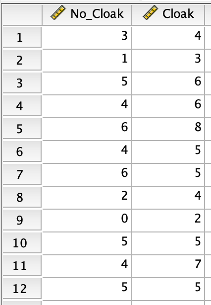
Think back to the data file for Statistics lecture 7 (“Comparing means - part 2”). In this file, one row corresponded to one participant, and for each participant you had two data points corresponding to the two conditions:

This type of file is what SPSS needs to run a paired-samples t-test: For a within-subjects design with two conditions, we need two data points for each participant, both in the same row.

Accordingly, for the flanker task you would need one data point for congruent trials and one data point for incongruent trials for each participant.

What we typically get from PsychoPy: Many rows per participant.

If your flanker task had, say, 72 experimental trials (half congruent, half incongruent), there would be 36 rows per condition in your PsychoPy output file! As SPSS expects one row per participant, we need a summary measure to represent the performance of each participant in both conditions. The remainder of this chapter and the next chapter explain one approach to obtaining this summary measure.

42.2 How to get from PsychoPy output to SPSS input

The simplest approach for creating our summary measure would be to simply calculate the mean RT for all trials from a condition and participant. However, this approach has the potential shortcomings listed below.

Extreme RTs

First, there might be extremely fast as well as extremely slow responses. Extremely fast responses (say, faster than 100-150 ms) are likely anticipatory responses. That is, participants anticipated the appearance of the stimulus and pressed a response key before properly processing the stimulus. Why 100-150 ms? The reason for this is that even in the macaque it takes about 70 ms on average for signals from the retina to arrive at the primary visual cortex (Lamme & Roelfsema, 2000)². In a choice reaction time task, once these signals arrive, lower and higher order visual processing areas must process the object identity (“Which target is it?”). Once the target has been identified, the correct response must be identified (e.g., “H requires a left-hand response”). Finally, a motor signal must be sent to an effector (i.e., a finger must press down one of the response keys). This is not to say that all of these processes occur strictly sequentially, but taking the various processing steps into account, it seems extremely unlikely that participants can produce valid responses (not just lucky guesses) before 100-150 ms (also see Whelan, 2008).

On the other hand, there might be extremely slow responses. These are likely due to lapses of attention or external distractions. Or, if your trials have infinite length, a participant might also have taken a break in the middle of your experiment! As these slow responses are not a direct consequence of the processing requirements of the task, an argument can be made for excluding them as well. The exact cut-off will be different for different tasks. For a straightforward flanker task run with healthy young participants, RTs which are longer than, say, 3 seconds might be considered extreme RTs.

Incorrect RTs

In addition, some of the trials were likely incorrect. There is very good evidence that error trials in this type of speeded reaction time task are faster than correct trials (e.g., Smith & Brewer, 1995). In addition, errors are more likely to occur on incongruent trials than on congruent trials (e.g., Derrfuss et al., 2021). If a simple averaging approach that includes all trials for each condition were taken, the overall estimates will be slightly off (because fast error trials are included). What is more, the incongruent trials would be affected more strongly (because there are more error trials in the incongruent condition), thus reducing the overall RT difference between congruent and incongruent trials and making it less likely to find a significant effect.³

Outlier RTs

Finally, there might be outlier RTs. The difference between extreme RTs and outlier RTs as used in the HHG is that the former are absolute, whereas the latter are relative to the other RTs from the same condition from the same participant.⁴ There are a number of ways to reject outlier RTs: The definition of outliers can be based on standard deviation, inter-quartile range, absolute median deviation, or simply a certain percentage of trials (e.g., 20% of the slowest and fastest trials are rejected).

For the purpose of our lab classes, we are only going to focus on SD-based outlier rejection. This is a pragmatic choice. SD-based outlier rejection has the disadvantage that the outliers themselves increase the SD, thus very strong outliers could potentially mask other outliers. On the other hand, SDs are easy to calculate and are good enough to illustrate the basic idea. In addition, a recent study (Berger & Kiefer, 2021) indicated that SD-based outlier rejection methods are actually relatively unbiased. That said, the Berger and Kiefer study was based on simulated data and it remains an open question how representative their simulated outliers are of real outliers. What’s more, another recent study came to the conclusion that when it comes to outlier rejection the cures might be worse than the disease (Miller, 2023). So, as you can see, the topic is still hotly debated. We believe you should at least know how to apply SD-based outlier rejection, so you can use it in the future if needed.

References

Berger, A., & Kiefer, M. (2021). Comparison of different response time outlier exclusion methods: A simulation study. Frontiers in Psychology, 12, e675558. https://doi.org/10.3389/fpsyg.2021.675558

Derrfuss, J., Danielmeier, C., Klein, T. A., Fischer, A. G., & Ullsperger, M. (2021). Unbiased post-error slowing in interference tasks: A confound and a simple solution. Behavior Research Methods, 54(3), 1416–1427. https://doi.org/10.3758/s13428-021-01673-8

Lamme, V. A. F., & Roelfsema, P. R. (2000). The distinct modes of vision offered by feedforward and recurrent processing. Trends in Neurosciences, 23(11), 571–579. https://doi.org/10.1016/s0166-2236(00)01657-x

Miller, J. (2023). Outlier exclusion procedures for reaction time analysis: The cures are generally worse than the disease. Journal of Experimental Psychology: General, 152(11), 3189–3217. https://doi.org/10.1037/xge0001450

Smith, G. A., & Brewer, N. (1995). Slowness and age: Speed-accuracy mechanisms. Psychology and Aging, 10(2), 238–247. https://doi.org/10.1037//0882-7974.10.2.238

Whelan, R. (2008). Effective analysis of reaction time data. The Psychological Record, 58(3), 475–482. https://doi.org/10.1007/BF03395630

---

1. If you can’t remember how exactly these measures of central tendency and dispersion are calculated, you might want to return to your statistics lectures and look this up.

2. Note that this is the very same Victor Lamme who co-founded Neurensics, the company behind the dubious “Girl with a Pearl Earring” study.

3. In fact, we recently showed that a very similar issue has been a confound in many publications investigating post-error slowing (Derrfuss et al., 2021).

4. Note that other people might use the terms “extremes” and “outliers” differently. Therefore, you should always define these terms if you use them.