58  SPSS basics

🏢 Lab class

58.1 Updates

As announced on the Moodle forum, the Wednesday 9am lab class was moved to Friday 2pm. As a result, all coursework deadlines this semester (except for the summative lab report) will be on Fridays at 4pm. We have updated the assessment overview in Chapter 6 and the module calendar accordingly.

Remember that Research Participation Scheme (RPS) points will contribute 10% to your overall module mark. Now is a great time to accumulate RPS points by participating in studies advertised on SONA!

This lab is an introduction to using SPSS. There won’t be that much new material (if you practised using SPSS for your statistics module!). The reason for covering not much new material is that we wanted to give those of you who haven’t completed working through the Excel material from last semester an opportunity to catch up. This is important as there will be an Excel quiz next week. Note that this quiz will have no time limit. We don’t want you to memorise Excel formulas, we want you to be able to apply them!

58.2 Installing SPSS

If you have not yet installed SPSS on your computer, please do so after the lab class (and use one of the iMacs during the lab class). To install SPSS on your computer, follow the instructions available in the section “Introduction to statistical software” of your statistics module on Moodle.

58.3 Background

Today, we are going to analyse data from an arrow flanker task and a Stroop task. We will analyse RTs and accuracies from congruent and incongruent trials of both tasks. A brief reminder about congruency in the flanker and the Stroop task (also see Chapter 21):

Task	Congruent	Incongruent
Arrow flanker task	→ → → → →	→ → ← → →
Stroop task	RED	BLUE

For our analyses, we will be using SPSS. The main aim for our first-year lab classes is that you get a good basic working knowledge of SPSS. We will focus on how to get data into SPSS, how to compute variables, how to screen data, and on how to run some basic analyses.

58.4 Getting help with SPSS

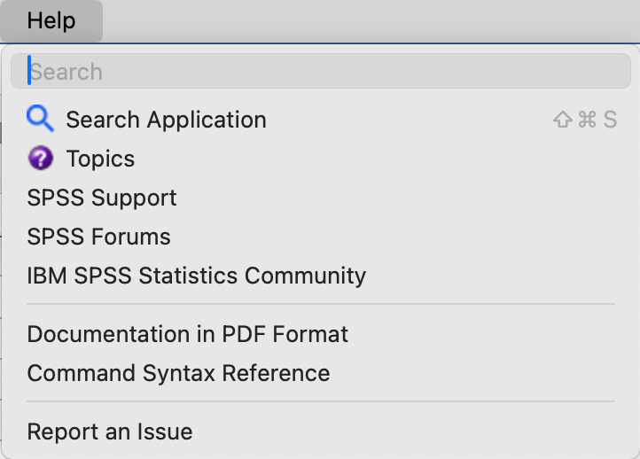
SPSS has a Help menu entry:

In addition, frequently there are context-sensitive help buttons on dialogue boxes:

Megan Barnard has set up a really useful Xerte toolkit for help with SPSS, the Statistical Analysis Support System.

In addition, IBM also offer a “brief” introductory SPSS guide (~ 90 p.) for download. In addition, many other resources are available on the internet (e.g., tutorials, videos, answers to specific questions). Finally, it would be a very good idea to get hold of a copy of Andy Field’s SPSS book.

That said, in many cases you’ll probably get a quicker answer by asking an AI tool. However, as always, make sure verify its accuracy against trusted sources.

58.5 Getting data into SPSS

58.5.1 Importing data

SPSS can import data from text files (e.g., .csv or .txt files), Excel files (.xlsx), and a number of other file types which need not concern us here. We will import data from a .csv file. The .csv file contains participant information and mean RTs from an arrow flanker task and a colour-word Stroop task.

I’ll demonstrate this now - you’ll have an opportunity to practise this when working on the exercise.

WarningmacOS users

If you are running macOS and use Safari, note that Safari likes to open .csv files directly in the browser. You could copy and paste the file contents into a text file and save it as a .csv files, but the easier solution probably is to use another browser instead (see Chapter 9).

To import the file, follow these steps: File → Import Data → select the appropriate file type and continue

As we have variable names at the top of the file, make sure that the appropriate option is selected. The import process should be pretty much straightforward.

After importing the .csv file, make sure to save the data file as a .sav file!

NoteShow/hide information on how this file was created

You might wonder how this file was created. After all, it contains the data of more than 150 participants! Of course, we did not do this manually. Instead, this was done using a [Python script]((https://github.com/jderrfuss/berrypy). The mean RT calculation was based on the following criteria:

• Only correct trials were taken into account.
• Extreme values were rejected.
  • Flanker: RTs below 150 ms and above 2000 ms
  • Stroop: RTs below 150 ms and above 2500 ms
• Outliers were rejected using the median absolute deviation (MAD; for details, see Leys et al., 2013).
  • Exclusion criterion for both tasks: values above or below 2.5 \(\times\) MAD (see Leys et al., 2013)
• Minimum trial number for mean calculation: 6 (i.e., if fewer than 6 trials remained after applying the criteria above, no mean was calculated)

58.5.2 Entering data

Manually entering data into SPSS is a pain. Avoid it if you can. If you really have to enter data manually, check them very carefully after entering them. It is very easy to make mistakes.

58.5.3 Opening existing data

Double-click on a .sav file. Alternatively, use File → Open → Data.

58.6 Types of files

SPSS knows three main types of files: data, syntax, and output files.

Data files

• Extension: .sav
• These files contain your data and associated information (e.g., variable names, variable labels).

Syntax files

• Extension: .sps
• These files contain SPSS syntax (i.e., commands to run analyses)
• If you have used the GUI to set up an analysis, clicking on Paste will open a syntax editor window and paste the command line equivalent of the analysis into it; if you save this file, you can later easily re-run an analysis
• SPSS will also add the syntax to the output (referred to as Log in the output Viewer window)

Output files

• Extension: .spv
• These files contain any output you have generated and saved (including analyses and graphs).

58.7 Types of windows

Associated with the three file types are three different types of windows.

Data editor window

To open a new data editor window, click on File → New → Data. This window will also open when you start SPSS.

There are three views within the Data editor window:

• Overview: We’ll ignore this one as it’s not terribly useful.

• Data View

  • As the name suggests, this is where you can view the data.
  • Usually, one row contains all the data from one participant (“one row, one participant rule”).
  • The columns are the variables.

• Variable View: You can find out more about the Variable View options available here and in the SPSS Knowledge Center.

It is always a good idea to use variable names that make it immediately clear what the variable actually is. stroop_RTcon is something you’ll probably be able to make sense of in the future. This might not be the case for something like strtc (although at the time it might feel a good acronym for stroop RTs congruent). In addition, you can add variable labels and value labels (more info about labels) that make it easier to remember what variable names and values mean.

Please note that having clear variable names will also allow you to easily work out which columns contain data from different levels of the same IV (in a within-subject design), and which columns contain data from different IVs.

Syntax editor window

We’re going to ignore syntax windows.

If you need one: File → New → Syntax

Viewer window

This window will also open when you open a data file or run an analysis. If you wanted to open a new one: File → New → Output

Note the outline in the frame on the left; you can use this outline to:

• Navigate the output → click on text label
• Hide output → click on arrow head
• Move parts of the output around → click and hold, then move
• Delete output → select and press delete

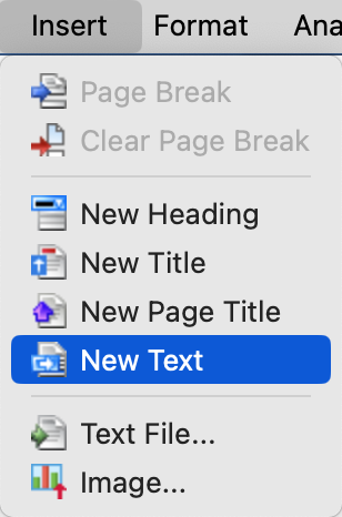
Please note that you can add additional information to the output. We recommend using this feature to remind you of the analysis you ran and why you ran it. To use this feature, the output window needs to be selected. You can then click on Insert in the menu bar and, e.g., insert comments using “New Text”:

58.8 Computing new variables

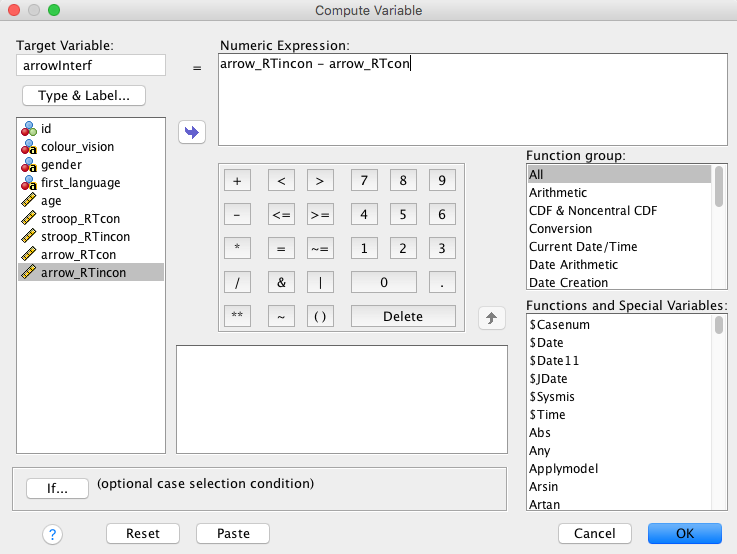
Please note that our data file only includes the condition-specific mean RTs. If we would also like have a measure of the size of the RT interference effect (i.e., the RT difference between incongruent and congruent trials), we will need to compute it. We will use the flanker task as an example. In SPSS, computing new variables is done by Transform → Compute Variable.

In our case, this computation is pretty straightforward. First, we define a name for the variable we would like to create (the “Target Variable” which we’ll call “arrowInterf”). Then, we add the two relevant existing variables to “Numeric expression” and make sure “arrowRTcon” is subtracted from “arrowRTincon” by adding a minus sign between them:

After clicking OK, you should find a new variable in your Data editor window. Note that new variables are always added to the right. This might mean that you need to scroll to the right to see the new variable.

Please note that SPSS allows for much more complex rules for computing new variables which we’re not going to cover. You might want to explore these possibilities at a later point in time (in his book, Andy Field talks about these possibilities in some detail).

🏠 Self-study

58.9 SPSS alternatives

Like any piece of software, SPSS has its advantages and disadvantages. SPSS will usually be fine for conducting a run-of-the-mill frequentist analysis. However, SPSS also tends to have some shortcomings:

• The SPSS graphical user interface (GUI) is sometimes not the easiest to use.
  • It can be difficult to find things (e.g., analyses, or analysis options).
  • The GUI might feel a bit dated.
• The output might not be the clearest you will come across.
• SPSS has been somewhat slow when it comes to integrating more recent statistical developments (e.g., confidence intervals or Bayesian analyses).
• If you have to pay for it, it is very expensive.

For these reasons and others it might be a good idea to at least be aware of the alternatives to SPSS. In fact, it might even be a good idea to become familiar with two statistical software packages.

Please see below for some free alternatives to SPSS. All of these are based on the statistical software R. We would encourage you to try out some of these and compare them to using SPSS.

Please do not forget that all statistical software packages share one major shortcoming: They can’t think. They will do whatever you tell them to do. They don’t care if the analysis makes sense or not. The analysis might run, the output might look plausible, but the analysis might be incorrect anyway. It’s up to you to decide if an analysis makes sense or not. SPSS (or any other statistical software) can’t make that decision for you. Therefore: First find out which analysis you should run, and then find out how to run it in whatever software you are using.

jamovi

jamovi is a relatively new statistical spreadsheet app designed to be easy to use. The jamovi user guide is available here. A great feature of jamovi is that its functionality can be extended by modules. For example, there is a module for Bayesian analyses. Note that there is a Chromebook and a cloud-based version available.

Please note that Megan’s Statistical Analysis Support System also covers jamovi!

JASP

JASP is a recently developed user-friendly statistical software package with one major advantage: It can run classical (i.e., frequentist) as well as Bayesian analyses. JASP support is available here. Note that there is a Chromebook version available.

RStudio

RStudio is an excellent integrated development environment for R. In fact, the Hitchhiker’s Guide was written using RStudio and Quarto.