Chapter 25 Introduction to data preprocessing
Over the past weeks we’ve looked at how to design, set up and run experiments. We’ve learned that PsychoPy creates an output file when we run an experiment (see Section 20). Now, it’s time to analyse these output files. This is where your statistics knowledge becomes relevant for the practicals: Using an example output file, we will calculate means, medians and standard deviations.33
25.1 What we get from PsychoPy and what we need for SPSS
Let’s return to our classic letter flanker task. Remember that on each trial there is a target that is relevant to the task and that next to the target there are irrelevant flankers. In the simplest version of the task, there might just be two letters that make up the stimuli. For example, participants might be required to press left when the target is “H” and right when the target is “S”. A congruent trial is when target and flankers require the same response (e.g. “SSSSS”), and an incongruent trial is when target and flankers require different responses (e.g., “SSHSS”). Imagine you completed a version of the task consisting of 72 trials, 36 of which were congruent and 36 incongruent, on PsychoPy. Accordingly, your output file has 72 rows corresponding to the experimental trials in the experiment.34
Let’s assume your aim is to find out if RTs on incongruent trials are on average significantly slower than RTs on congruent trials. To investigate this, you would collect data from a sample and run an inferential statistical test on the condition means. Remember that this is a within-subject design, as the same participants complete all levels of the IV, so eventually (after checking test assumptions) you might decide that a paired-samples t-test is appropriate.
Now think back to the Activity 6 data file for Statistics lecture 7 (Comparing means - part 2). In this file, one row corresponded to one participant, and for each participant you had two data points corresponding to the two conditions:
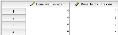
This type of file is what SPSS needs to run a paired-samples t-test. That is, for a within-subjects design with two conditions, we need two data points for each participant. However, at present we have 36 data points for each participant and condition! That is, we have 36 RTs from congruent trials and 36 RTs from incongruent trials. How do we get from 36 to one? Clearly, what we need is some sort of summary measure to represent performance in both conditions.
25.2 How to get from PsychoPy output to SPSS input
The simplest approach for creating our summary measure would be to simply calculate the mean RT for all trials from a condition and participant. However, this approach has potential shortcomings listed below.
Extreme RTs
First, there might be extremely fast as well as extremely slow responses. Extremely fast responses (say, faster than 100-150 ms) are likely anticipatory responses. That is, participants anticipated the appearance of the stimulus and pressed a response key before properly processing the stimulus. Why 100-150 ms? The reason for this is that even in the macaque it takes about 70 ms on average for signals from the retina to arrive at the primary visual cortex (Lamme & Roelfsema, 2000). In a choice reaction time task, once these signals arrive, lower and higher order visual processing areas must process the object identity (“Which target is it?”). Once the target has been identified, the correct response must be identified (e.g., “H requires a left-hand response”). Finally, a motor signal must be sent to an effector (i.e., a finger must press down one of the response keys). This does not necessarily mean that all of these processes occur strictly sequentially, but taking the various processing steps into account, it seems extremely unlikely that participants can produce valid responses (not just lucky guesses) before 100-150 ms.
On the other hand, there might be extremely slow responses. These are likely due to lapses of attention or external distractions. Or, if your trials have infinite length, a participant might also have taken a break in the middle of your experiment! As these slow responses are not a direct consequence of the processing requirements of the task, an argument can be made for excluding them as well. The exact cutoff will be different for different tasks. For a straightforward flanker task run with healthy young participants, RTs which are longer than, say, 3 seconds might be considered extreme RTs.
Incorrect RTs
In addition, some of the trials were likely incorrect. There is very good evidence that error trials in this type of speeded reaction time task are faster than correct trials (e.g., Smith & Brewer, 1995). In addition, errors are more likely to occur on incongruent trials than on congruent trials (e.g., Derrfuss et al., 2021). If a simple averaging approach that includes all trials for each condition were taken, the overall estimates will be slightly off (because fast error trials are included). What is more, the incongruent trials would be affected more strongly (because there are more error trials in the incongruent condition), thus reducing the overall RT difference between congruent and incongruent trials and making it less likely to find a significant effect.35
Outlier RTs
Finally, there might be outlier RTs. The difference between extreme RTs and outlier RTs is that the former are absolute, whereas the latter are relative to the other RTs from the same condition from the same participant.36 There are a number of ways to reject outlier RTs: The definition of outliers can be based on standard deviation, inter-quartile range, absolute median deviation, or simply a certain percentage of trials (e.g., 20% of the slowest and fastest trials are rejected). For the purpose of our lab classes, we are only going to focus on SD-based outlier rejection. This is a pragmatic choice. SD-based outlier rejection is not ideal due to the fact that the outliers themselves increase the SD. On the other hand, SDs are easy to calculate and are good enough to illustrate the basic idea.
References
If you can’t remember how exactly these measures of central tendency and dispersion are calculated, you might want to return to your statistics lectures and look this up.↩︎
There will also be a header row and there might be rows corresponding to other routines in the task or to practice trials. Let’s ignore these for now and focus only on the experimental trials.↩︎
In fact, our recent paper (Derrfuss et al., 2021) makes the point that a very similar issue has been a confound in many publications investigating post-error slowing.↩︎
Note that other people might use the terms “extremes” and “outliers” differently. Therefore, you should always explicitly say what you mean.↩︎