Chapter 27 Data preprocessing with R
In this chapter, we will show you how to apply the same preprocessing steps in R. You do not need to work through the R code if you’re not interested in how R works. We only show this for the students who are. If you’d like to see the R code, click on the “Show code” buttons. Note that the results are identical to those obtained with Excel.
library(tidyverse)

# read csv file
data <- read_csv("./assets/lab10_flanker_output_file/1_1_letter_flanker.csv")

# remove practice trials and create ms RT column
data <- data %>%
  filter(trials.thisN >= 0) %>%  # only keep main trials loop
  mutate(rt_ms = response.rt * 1000) # create new column with RTs in ms

# calculate overall accuracy (including extreme trials)
overall_acc = summarise(data, (sum(response.corr == 1) / (sum(response.corr == 1 | response.corr == 0))))
overall_acc = unlist(round(overall_acc * 100, digits = 1))  # multiply by 100, round to 1 digit, turn into double (summarise returns list)

# filter out extremes
data_no_extr <- data %>%
  filter(rt_ms >= 150, rt_ms <= 3000)

# calculate percentage of extreme trials
nr_extr = nrow(data) - nrow(data_no_extr)  # nr of rows in data minus nr of rows in data_no_extr
percent_extr = round((nr_extr/nrow(data)) * 100, digits = 1)

# calculate accuracies per condition (including outliers)
condition_acc <- data_no_extr %>%
  group_by(congruency) %>%
  summarise(accuracy = (sum(response.corr == 1)/(sum(response.corr == 1 | response.corr == 0)))) %>%
  mutate(accuracy = round(accuracy * 100, digits = 1))

# keep only correct trials
data_no_extr_only_corr <- data_no_extr %>%
  filter(response.corr == 1)

# calculate mean RTs per condition without outlier removal and median RTs
mean_rts_with_outl <- data_no_extr_only_corr %>%
  group_by(congruency) %>%
  summarise(mean_w_outl = round(mean(rt_ms, na.rm=TRUE), digits = 0),
            median = round(median(rt_ms, na.rm=TRUE), digits = 0)
  )

# calculate thresholds for outlier removal
outl_thresh <- data_no_extr_only_corr %>%
  group_by(congruency) %>%
  summarise(lthresh = mean(rt_ms, na.rm=TRUE) - (2. * sd(rt_ms, na.rm=TRUE)),
            uthresh = mean(rt_ms, na.rm=TRUE) + (2. * sd(rt_ms, na.rm=TRUE))
  )

# add the outlier removal thresholds to the tibble
# con trials will get con thresholds, incon trials incon thresholds
# this is done to allow the filtering operation in the next step
data_no_extr_only_corr_with_thr <- full_join(data_no_extr_only_corr, outl_thresh, col = "congruency")

# remove outliers using the thresholds
data_no_extr_only_corr_no_outl <- data_no_extr_only_corr_with_thr %>%
  filter(rt_ms >= lthresh, rt_ms <= uthresh) # keep trials between +/- 2 SDs

# calculate mean RTs per condition with outlier removal
mean_rts_no_outl <- data_no_extr_only_corr_no_outl %>%
  group_by(congruency) %>%
  summarise(mean_no_outl = round(mean(rt_ms, na.rm=TRUE), digits = 0))

# combine results not distinguishing between con and incon trials
resultsOverall <- as_tibble(cbind(overall_acc, percent_extr))
print(resultsOverall)
## # A tibble: 1 × 2
## overall_acc percent_extr
## <dbl> <dbl>
## 1 93.1 2.8# combine results into one tibble
results <- list(condition_acc, mean_rts_with_outl, mean_rts_no_outl) %>%
reduce(left_join) %>% # join list of tibbles
relocate(median, .after = last_col()) # move median column to the right
print(results)## # A tibble: 2 × 5
## congruency accuracy mean_w_outl mean_no_outl median
## <chr> <dbl> <dbl> <dbl> <dbl>
## 1 con 97.2 484 475 456
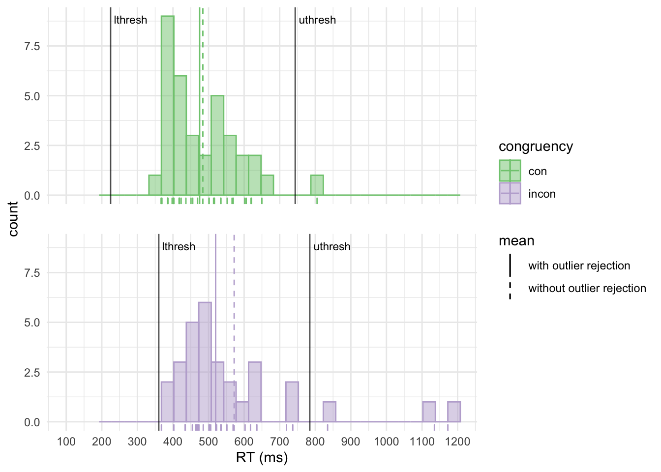
## 2 incon 88.2 572 531 504One of the advantages of using R is that it has a powerful visualisation package called ggplot2. Using ggplot2, the content and layout of plots can be controlled using code. This is far superior to visualisations in Excel, which typically have very limited options and frequently require manual interventions.
Let’s plot our RT distributions using ggplot2. Note how the visualisations make it intuitively clear how the RTs are distributed, where the lower and upper outlier rejection thresholds are and how outlier rejection affects the condition means.
library(ggplot2)

# rearrange the thresholds tibble (necessary for plotting with geom_vline)
outl_thresh2 <- outl_thresh %>%
  pivot_longer(
    cols = c("lthresh", "uthresh"),
    names_to = "threshType",
    values_to = "thresh"
  )

# plot the RT distributions
ggplot() +
  geom_histogram(data = data_no_extr_only_corr, aes(x = rt_ms, fill = congruency, colour = congruency),
                 position = "identity", alpha = 0.5, binwidth = 35) +  # add histogram
  scale_color_brewer(palette="Accent") +  # change outline colours
  scale_fill_brewer(palette="Accent") +   # change fill colours
  geom_rug(data = data_no_extr_only_corr, aes(x = rt_ms, colour = congruency)) +  # add rug plot
  geom_vline(data = mean_rts_with_outl, aes(xintercept = mean_w_outl, colour = congruency,
                                            linetype = "without outlier rejection")) +  # add means without outlier rejection
  geom_vline(data = mean_rts_no_outl, aes(xintercept = mean_no_outl, colour = congruency,
                                          linetype = "with outlier rejection")) +  # add means with outlier rejection
  scale_linetype_manual(name = "mean", values = c("with outlier rejection" = "solid",
                                                  "without outlier rejection" = "dashed")) +  # make one solid, the other dashed
  geom_vline(data = outl_thresh2, aes(xintercept = thresh), colour = "black", alpha = 0.7) +  # add outlier thresholds
  geom_text(data = outl_thresh2, aes(x = thresh, label = threshType),
            y = Inf, vjust = 2, hjust = -0.1, size = 3) +  # label outlier thresholds
  facet_wrap(vars(congruency), ncol = 1) +  # plot separate graphs for con and incon
  coord_cartesian(xlim = c(100, 1200)) +  # see https://github.com/tidyverse/ggplot2/issues/4083
  scale_x_continuous(name="RT (ms)", breaks = seq(from = 100, to = 1200, by = 100)) +  # x axis tick labels every 100 ms
  theme_minimal() +
  theme(strip.text = element_blank(), panel.spacing.y = unit(.8, "cm"))  # remove headers, increase spacing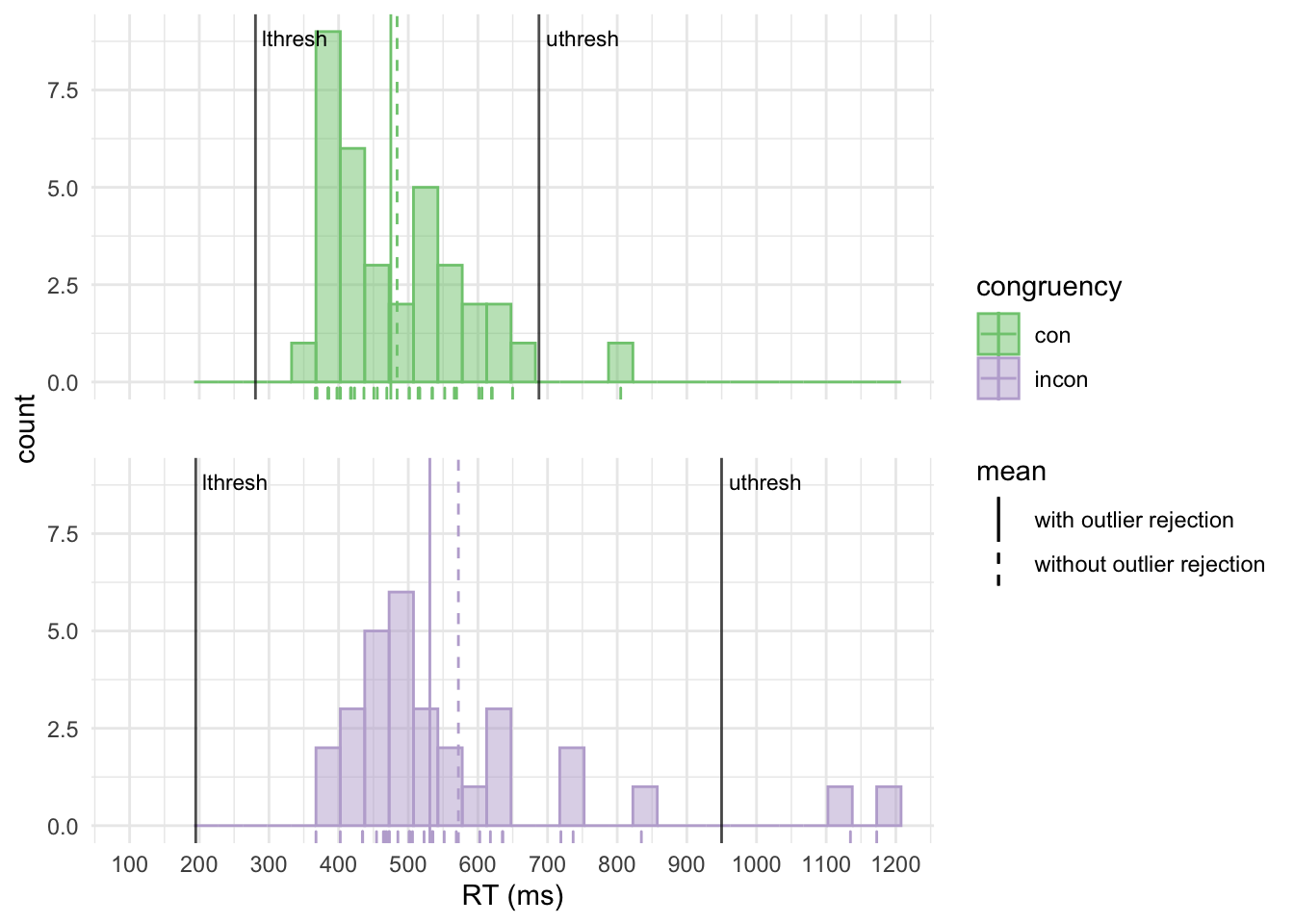
Let’s see what happens if we use the median absolute deviation (MAD) for outlier rejection.
library(tidyverse)

# read csv file
data <- read_csv("./assets/lab10_flanker_output_file/1_1_letter_flanker.csv")

# remove practice trials and create ms RT column
data <- data %>%
  filter(trials.thisN >= 0) %>%  # only keep main trials loop
  mutate(rt_ms = response.rt * 1000) # create new column with RTs in ms

# calculate overall accuracy (including extreme trials)
overall_acc = summarise(data, (sum(response.corr == 1) / (sum(response.corr == 1 | response.corr == 0))))
overall_acc = unlist(round(overall_acc * 100, digits = 1))  # multiply by 100, round to 1 digit, turn into double (summarise returns list)

# filter out extremes
data_no_extr <- data %>%
  filter(rt_ms >= 150, rt_ms <= 3000)

# calculate percentage of extreme trials
nr_extr = nrow(data) - nrow(data_no_extr)  # nr of rows in data minus nr of rows in data_no_extr
percent_extr = round((nr_extr/nrow(data)) * 100, digits = 1)

# calculate accuracies per condition (including outliers)
condition_acc <- data_no_extr %>%
  group_by(congruency) %>%
  summarise(accuracy = (sum(response.corr == 1)/(sum(response.corr == 1 | response.corr == 0)))) %>%
  mutate(accuracy = round(accuracy * 100, digits = 1))

# keep only correct trials
data_no_extr_only_corr <- data_no_extr %>%
  filter(response.corr == 1)

# calculate mean RTs per condition without outlier removal and median RTs
mean_rts_with_outl <- data_no_extr_only_corr %>%
  group_by(congruency) %>%
  summarise(mean_w_outl = round(mean(rt_ms, na.rm=TRUE), digits = 0),
            median = round(median(rt_ms, na.rm=TRUE), digits = 0)
  )

# calculate thresholds for outlier removal
outl_thresh <- data_no_extr_only_corr %>%
  group_by(congruency) %>%
  summarise(lthresh = mean(rt_ms, na.rm=TRUE) - (2.5 * mad(rt_ms, na.rm=TRUE)),  # see Leys et al., 2013
            uthresh = mean(rt_ms, na.rm=TRUE) + (2.5 * mad(rt_ms, na.rm=TRUE))
  )

# add the outlier removal thresholds to the tibble
# con trials will get con thresholds, incon trials incon thresholds
# this is done to allow the filtering operation in the next step
data_no_extr_only_corr_with_thr <- full_join(data_no_extr_only_corr, outl_thresh, col = "congruency")

# remove outliers using the thresholds
data_no_extr_only_corr_no_outl <- data_no_extr_only_corr_with_thr %>%
  filter(rt_ms >= lthresh, rt_ms <= uthresh) # keep trials between +/- 2 SDs

# calculate mean RTs per condition with outlier removal
mean_rts_no_outl <- data_no_extr_only_corr_no_outl %>%
  group_by(congruency) %>%
  summarise(mean_no_outl = round(mean(rt_ms, na.rm=TRUE), digits = 0))

# combine results not distinguishing between con and incon trials
resultsOverall <- as_tibble(cbind(overall_acc, percent_extr))
print(resultsOverall)
## # A tibble: 1 × 2
## overall_acc percent_extr
## <dbl> <dbl>
## 1 93.1 2.8# combine results into one tibble
results <- list(condition_acc, mean_rts_with_outl, mean_rts_no_outl) %>%
reduce(left_join) %>% # join list of tibbles
relocate(median, .after = last_col()) # move median column to the right
print(results)## # A tibble: 2 × 5
## congruency accuracy mean_w_outl mean_no_outl median
## <chr> <dbl> <dbl> <dbl> <dbl>
## 1 con 97.2 484 475 456
## 2 incon 88.2 572 520 504Note that the thresholds for incongruent trials are now much closer together and an additional trial is considered an outlier. This illustrates a problem with the SD-based approach: The outliers themselves increase the SD. Thus outliers might not be detected because there might be even more pronounced outliers that mask them. The MAD is not sensitive to outliers, thus does not suffer from this problem.
library(ggplot2)

# rearrange the thresholds tibble (necessary for plotting with geom_vline)
outl_thresh2 <- outl_thresh %>%
  pivot_longer(
    cols = c("lthresh", "uthresh"),
    names_to = "threshType",
    values_to = "thresh"
  )

# plot the RT distributions
ggplot() +
  geom_histogram(data = data_no_extr_only_corr, aes(x = rt_ms, fill = congruency, colour = congruency),
                 position = "identity", alpha = 0.5, binwidth = 35) +  # add histogram
  scale_color_brewer(palette="Accent") +  # change outline colours
  scale_fill_brewer(palette="Accent") +   # change fill colours
  geom_rug(data = data_no_extr_only_corr, aes(x = rt_ms, colour = congruency)) +  # add rug plot
  geom_vline(data = mean_rts_with_outl, aes(xintercept = mean_w_outl, colour = congruency,
                                            linetype = "without outlier rejection")) +  # add means without outlier rejection
  geom_vline(data = mean_rts_no_outl, aes(xintercept = mean_no_outl, colour = congruency,
                                          linetype = "with outlier rejection")) +  # add means with outlier rejection
  scale_linetype_manual(name = "mean", values = c("with outlier rejection" = "solid",
                                                  "without outlier rejection" = "dashed")) +  # make one solid, the other dashed
  geom_vline(data = outl_thresh2, aes(xintercept = thresh), colour = "black", alpha = 0.7) +  # add outlier thresholds
  geom_text(data = outl_thresh2, aes(x = thresh, label = threshType),
            y = Inf, vjust = 2, hjust = -0.1, size = 3) +  # label outlier thresholds
  facet_wrap(vars(congruency), ncol = 1) +  # plot separate graphs for con and incon
  coord_cartesian(xlim = c(100, 1200)) +  # see https://github.com/tidyverse/ggplot2/issues/4083
  scale_x_continuous(name="RT (ms)", breaks = seq(from = 100, to = 1200, by = 100)) +  # x axis tick labels every 100 ms
  theme_minimal() +
  theme(strip.text = element_blank(), panel.spacing.y = unit(.8, "cm"))  # remove headers, increase spacing