Chapter 35 Rejecting outliers based on SDs

You will find that some sections below have a grey background. This is in-depth information that goes beyond what will be required for the lab report, but is good to be aware of.

This chapter covers how to remove outliers based on SDs in SPSS. For this step, we will again use the data from the flanker and the Stroop task. The SPSS data file below already includes the RT interference scores.

Please download the SPSS data file and open it in SPSS.

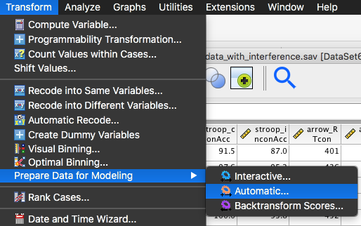
Initially, we need to go to Transform → Prepare Data for Modeling → Automatic:

Using “Prepare Data for Modeling” for this purpose is a bit like using a sledgehammer to crack a nut, but it is nevertheless the most straightforward approach within SPSS.

The window that opens after clicking on “Automatic” has three different tabs, “Objective”, “Fields” and “Settings”. We will look at these in turn.

Objective

You can simply leave the default “Balance speed & accuracy” setting. (Note that SPSS will change this to “Customize Analysis” automatically.)

Fields

Remove all variables except interfArrowRT and interfStroopRT from the “Inputs” field.

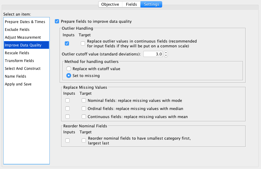
Settings

Unselect all of the following (we can ignore “Prepare Dates & Times”):

The only option where we need to change settings is “Improve Data Quality”. We are going to use 3 SDs for outlier rejection for this analysis and we will set outliers to missing:

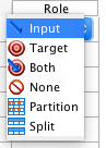
If you run the analysis and SPSS complains about there not being a “nominal target”, go to Variable View and check what is referred to as the role of the variables. If the role looks like this, SPSS will complain:

Change the role:

The result should look like this:

You might find that SPSS resets these values to “None” after you’ve run the analysis. Note that this will not affect the Frequencies output below.

After running the analysis, we have two new variables, interfArrowRT_transformed and interfStroopRT_transformed. Note that in your Data View SPSS will add these to the right of your existing variables, so you might need to scroll to the right for the new variables to become visible.

We can re-run Frequencies to check how the outlier rejection has affected descriptive statistics. We find that the outlier rejection had a very small effect on the mean. As expected, outlier rejection somewhat reduces the SD and the SE:

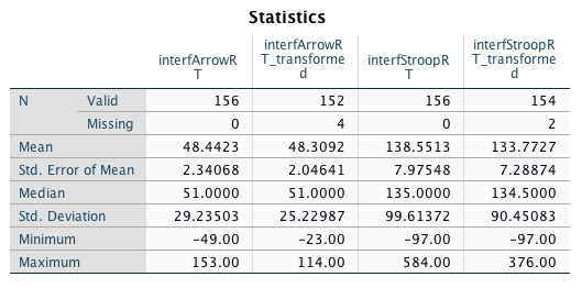
However, we also note that the minimum value for the Stroop task has not changed. A negative interference effect of -97 ms was within 3 SDs of the mean interference effect in the Stroop task. A simple calculation shows that only negative interference effects below -160 ms would have been rejected:

\[138.6 - 3 * 99.6 = -160.2\]

Apart from the previously mentioned problem that outliers themselves increase the SD and that therefore the median absolute deviation (MAD) is often a better choice, another problem becomes apparent (and one that using the normal MAD does not solve either): the rejection criteria are symmetric around the mean. That is a value of 3 SDs below the mean is treated exactly the same way as a value of 3 SDs above the mean. An argument can be made that values on both sides of the mean should not be treated in the same way if the distributions are not symmetrical, and that separate SD-based or MAD-based rejection thresholds should be calculated for values below and above the mean. If you are interested in this approach, you can read more about it on this webpage on using the double MAD approach.