Chapter 23 Excel formulas and functions
23.1 Formulas
Important basics about formulas in Excel:
- Formulas in Excel always begin with an equals sign:
= - The formula is always typed into the cell where the answer should appear
- The formula is completed by pressing
Enteron the keyboard
23.1.1 Basic arithmetic operators
Below are some examples for formulas using arithmetic operators.
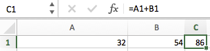
Add the values in cells A1 and B1: =A1+B1
To get the answer in C1:
Subtract the value in B1 from the value in A1: =A1-B1
Multiply the values in cells A1 and B1: =A1*B1
You get the idea. More information on operators from Microsoft.
23.2 Functions
Formulas can make use of predefined functions in Excel. We will only describe a very small set of functions that will be fundamental to our analyses. For more information, see this page about Excel functions sorted by category or this page about Excel functions in alphabetical order.
If you want help on functions in Excel, click on the function symbol \(fx\):

This will open the Formula Builder, providing you with information on the available functions, and if you double-click on a specific function, help with building the formula. Alternatively, go to “Help” → “Excel Help”, or search online.
23.2.1 IF
IF is one of the most important logical functions in Excel. It works in the following way:
IF(something is True, then do something, otherwise do something else)
So an IF statement can have two results. The first result is if your comparison is True, the second if your comparison is False. A typical use case for this function is to create a column of values that includes only correct RTs.
Imagine you have the following PsychoPy output:
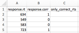
The first column contains all RTs, and the second column information about accuracy (remember that PsychoPy codes correct responses as 1, and incorrect responses as 0). Your aim is to have only RTs associated with correct responses in your third column.
You can use the following formula in cell C2 to achieve this:
=IF(B2=1, A2, "")
This states that:
- If
B2equals 1 (i.e., if the trial is correct)- Then
C2should be equal toA2(basically copying the value fromA2toC2)
- Then
- If this is not the case (i.e., if the trial is not correct) [this part is implicit to the function]
- Then
C2should remain empty (indicated by"")
- Then
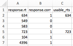
If we apply this formula to all rows in our worksheet (by copying it to the adjacent cells), we get the following output:

Column C now only contains RTs associated with correct trials.
Note that you can create more complex statements by combining multiple conditions using AND or OR. For example, you might not only want to remove RTs from incorrect trials, but also RTs that are extremely fast (presumably representing anticipatory responses) or extremely slow (presumably representing lapses of attention), independent of their accuracy. Based on previous research, you might consider RTs below 150 ms as anticipatory, and RTs over 4000 ms as lapses of attention. You could use the following formula to achieve your aim:
=IF(AND(B2=1, A2>=150, A2<=4000), A2, "")
This states that:
- If
B2equals 1 and A2 is equal to or above 150 ms and A2 is equal to or less than 4000 ms- Then
C2should be equal toA2(basically copying the value fromA2toC2)
- Then
- If this is not the case
- Then
C2should remain empty (indicated by"")
- Then
Result:
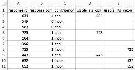
Quite frequently, you will take into account an additional column indicating the condition. For example, there might be an additional column coding the congruency of the stimulus, with the levels con and incon. If you wanted to have separate columns for your congruent and incongruent RTs, you could do this as illustrated below.
For the column with all congruent RTs:
=IF(AND(B2=1, A2>=150, A2<=4000, C2="con"), A2, "")
For the column with all incongruent RTs:
=IF(AND(B2=1, A2>=150, A2<=4000, C2="incon"), A2, "")
Please note that letter strings need to be in quotes.
Result:
23.2.2 SUM
SUM is another relevant function. You can add individual values, cell references or ranges or a mix of all three.
For example:
=SUM(A2:A10)
=SUM(A2:A10, C2:C10)
23.2.3 AVERAGE
AVERAGE is another function you will frequently need. It returns the average (arithmetic mean) of the arguments. For example, if the range A1:A20 contains numbers, the formula =AVERAGE(A1:A20) returns the average of those numbers.
Please note that the value 0 will be treated like any other number by this function (thus affecting your mean!), whereas empty cells are ignored.
Variants of AVERAGE are AVERAGEIF and AVERAGEIFS. These variants allow the specification of one or multiple conditions that must be met in order for numbers to be averaged.
23.2.4 Other functions
Other potentially relevant functions are:
IFS: test multiple conditions and return a value corresponding to the first TRUE result; unlike the IF function, IFS allows you to test more than one condition without nestingCOUNT: count cells with numbers; will not count empty cells, logical values, text, or error valuesCOUNTA: count cells with logical values, text, or error values; will not count empty cellsCOUNTIF: count cells dependent on the outcome of a logical testCOUNTIFS: count cells dependent on the outcomes of multiple logical testsROWS: returns the number of rows in a rangeMEDIAN: calculate the medianSTDEV.S: standard deviation of a sampleCORREL: correlation
More details about all these function can be found in the Excel help and online.
23.3 Copying formulas
Formulas can be copied to adjacent cells using what Excel calls the “fill handle”:
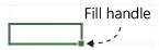
If you place your mouse cursor over the fill handle, it will turn into a plus sign. If you now drag the fill handle, you can copy formulas to adjacent cells. Note that this will update relative cell references. For example, if you copy the formula =A1+B1 from row 1 to row 2, the formula will become =A2+B2. Typically, this is the behaviour you want. However, sometimes, you might want to, for example, subtract a value in a specific cell from other values. For example, you might have calculated the mean for some values and now you would like to calculate the deviation from the mean (i.e., to subtract the mean from your other values.)
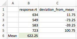
This is when absolute cell references (see Section 22.8) are required. Use the following formula in cell C2 to subtract the mean from all values: =B2-$B$6 (where $B$6 is the absolute reference to cell B6)
When you copy this formula downwards, only the first cell reference will be updated. That is, the formulas will become:
- Row 3:
=B3-$B$6 - Row 4:
=B4-$B$6, etc.
If you want to re-use a formula in a new cell without changing anything initially, the following procedure often works best:
- Select the cell with the to-be-copied formula
- Select the formula in the formula bar (the field next to \(fx\))
- Press
Cmd + CorCtrl + C - Press
Esc(don’t forget this step!) - Click on the cell to which the formula should be copied
- Press
Cmd + VorCtrl + V