Chapter 36 The one-sample t-test
You will find that some sections have a grey background. This is in-depth information that goes beyond what will be required for the lab report, but is good to be aware of.
This chapter will cover how to run a one-sample t-test using SPSS. As running the t-test is relatively straightforward, we will focus on understanding the output. We will also show you to how to report the t-test in a lab report following APA style.
The one-sample t-test tests if a mean observed in a sample is significantly different from a mean expected under the null hypothesis. Typically, the mean expected under the null will be 0. For us, the one-sample t-test will find out if there was a significant interference effect in the flanker task. We will use a traditional \(\alpha\) of .05, but note that there have been recent calls for stricter \(\alpha\) levels to be used within psychology.
Please download this SPSS data file and open it in SPSS.
Please note that we will be using relatively small sets of data with no outliers as this will make the subsequent step-by-step analyses in Excel easier.
36.1 Running the one-sample t-test
To run a one-sample t-test in SPSS, go to Analyze → Compare Means → One-Sample T Test

The “Test Value” refers to value you are testing against (the value expected under the null hypothesis).
Options
- Options
- The default 95% is the typical choice for Confidence Interval Percentage
- Missing Values
- This is only relevant if you have more than one variable (e.g., when you analyse both flanker and Stroop interference scores at the same time)
- Exclude cases analysis by analysis: A case that has a missing value for one variable (e.g., for the Stroop task) will still be included in the analysis for the second variable (e.g., the flanker task) → this is usually what you want
- Exclude cases listwise: As soon as there is one value missing, the participant will be excluded from all analyses (e.g., if the Stroop interference score is missing, they will also be excluded from the flanker analysis)
- Bootstrap: Not currently of interest
- Estimate effect sizes: You should tick the corresponding box.
36.2 The one-sample t-test SPSS output
The SPSS output consists of three tables. The first table includes descriptive statistics:
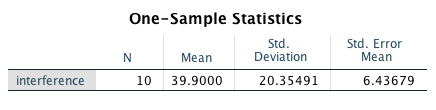
This table will be the basis for reporting some of the descriptive statistics required for your lab report.
The second table reports the t-test results:
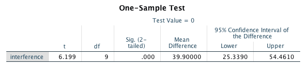
You need to include all of the information in this table in your lab report:
- The t-value
- The degrees of freedom (df in the table)
- The p-value (Sig. (2-tailed) in the table)
- The 95% confidence interval for the mean
Note: Running a one-sample t-test on the difference scores of two variables is mathematically identical to running a paired-samples t-test on the variables themselves. For example, running a one-sample t-test for the flanker RT difference scores (when using the raw RT differences as opposed to the percent interference scores) is identical to running a paired-samples t-test for flanker congruent and incongruent mean RTs. You can easily confirm this by running Analyze → Compare Means → Paired-Samples T Test on congruent and incongruent RTs.
Because the formulas for the one-sample t-test are much simpler, we focus on the one-sample t-test in the lab. The paired-samples t-test is explained in detail in Andy Field’s book.
The third table includes information about effect sizes:
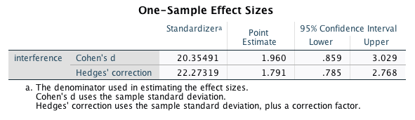
We will focus on Cohen’s d below as it straightforward to calculate. You can read more about Hedges’ correction in this article.
36.3 Interpreting the output
The t-value
The formula for the one-sample t-test is:
\[{t = \frac{\overline{x}}{s\frac{1}{\sqrt{N}}}}\]
where \(\overline{x}\) is the mean interference effect, \(s\) is the standard deviation, and \(N\) is the sample size.
Remember that the standard deviation is calculated in this way:
\[\large{s = \sqrt{\frac{\Sigma_{i=1}^N (x_i - \overline{x})^2}{N-1}}}\]
In words:
- For each value, calculate the deviation from the mean
- Square the deviation
- Sum up the squared deviations
- Divide the sum of the squared deviations by \(N-1\) (the result is the variance)
- Take the square root of the variance to get the standard deviation
As \(s\frac{1}{\sqrt{N}}\) is the standard error, the t-value formula can also be written as:
\[{t = \frac{\overline{x}}{SE}}\]
The calculation:
\[{t = \frac{39.9}{6.44}} = 6.2\]
Same t-value as in the SPSS output - great!
As a rule of thumb, if \(\alpha = .05\), the t-value needs to be more extreme than \(\pm2\) for the effect to be significant (the sign is irrelevant for two-tailed tests). Put differently, your empirically observed mean needs to be at least 2 standard errors away from 0 for the effect to be significant.
In our example, the t-value is approximately 6, meaning that our observed mean difference is roughly 6 standard error units away from the mean of 0!
The degrees of freedom
For a one-sample t-test, the degrees of freedom are the number of participants minus 1 (i.e., \(N-1\)).
The p-value
The p-value is an area associated with a particular t-value. It is the size of the area under the t-distribution which corresponds to the probability of observing the effect you observed or a more extreme one (assuming that the null hypothesis is true). If the size of this area is below .05 (i.e., if the area is less than 5% of the total area under the distribution), the effect is significant.
The p-value from our study is .000159. You can get this value…
by double-clicking on the table with the p-value in the output viewer and by double-clicking again on the p-value in the new window that opened after you first double-clicked, or
by double-clicking on the table with the p-value in the output viewer and hovering the mouse pointer over the p-value:

All very intuitive… This value is clearly smaller than .05, confirming that our result is significant.
The confidence interval
The confidence interval (CI) is reported as a range of values around the mean. It is meant to give the reader an approximate idea of how precise the estimate of the mean is. For our mean interference effect, SPSS reports that the lower limit of the 95% CI is 25 ms, and the upper limit is 54 ms.
How are these values calculated? We need to know three things to calculate the limits of the confidence interval:
- The mean (\(\overline{x}\))
- The standard error of the mean (\(SE\))
- The critical t-value (\(t_{crit}\))
The formula for the CI limits is:
\[CI\ limits = \overline{x} \pm SE * t_{crit}\]
If we would like to manually calculate the confidence interval, we can use a number of online calculators to look up the critical t-value (e.g., here). Using the online t-value calculator, we find that the critical t-value for 9 degrees of freedom, a probability level of .05 and two-tailed test is ±2.262 (i.e., roughly 2 → remember the rule of thumb!). We can now manually calculate the CI:
\[CI_{lower\ limit} = 39.9 - 6.44 \times 2.262 = 25.3\]
\[CI_{upper\ limit} = 39.9 + 6.44 \times 2.262 = 54.5\]
Exactly what SPSS calculated for us - hooray!
36.4 Lab 13 Exercise
In this exercise, you will compute a t-test step by step. The Excel file below includes the same data as the SPSS file, plus an additional 10 participants. First, make sure you understand the individual steps of the analysis for the first 10 participants. Then, compute your own t-test for the participants with the IDs 12 to 21. Check your result by copying the interference scores into SPSS and running a one-sample t-test on them.
Please download the file for the exercise and open it in Excel.
Here is a video of Jonathan completing the exercise:
Please note that the confidence interval tells you something about the statistical test: If the confidence interval includes 0, the result will not be significant, if it does not include 0, the result will be significant. Why is this? You can think about this in the following way: When is my result significant? When my t-value is below -2.262 or when my t-value is above 2.262. Remember that this means that for the result to be significant, my observed mean difference needs to be 2.262 SE units away from 0. We know that the SE of our distribution is 6.4 ms. Thus, we can express the same thing using our original units: To be significant, our mean difference needs to be below \(6.4 \times -2.262 = -14.5\ ms\) or above \(6.4 \times 2.262 = 14.5\ ms\). All the confidence interval then does is centre this range on the observed mean difference. Our lower limit will be \(39.9 - 14.5\), and our upper limit will be \(39.9 + 14.5\). Therefore, saying that the result is significant if the observed mean difference is more extreme than \(\pm14.5\) is the same thing as saying that the result is significant if 0 lies outside the observed mean difference \(\pm14.5\).
While the APA highly recommends the use of confidence intervals, their correct interpretation is tricky for students as well as researchers as has been shown by Hoekstra et al. (2014) (see also this comment and the rebuttal).
This is the correct interpretation of 95% confidence intervals for a t-test: Over a very large number of replications of a study, 95% of the confidence intervals will include the true mean difference. Technically, all of the following statements are not correct (see Hoekstra et al., 2014):
- The probability that the true mean is greater than 0 is at least 95%.
- The probability that the true mean equals 0 is smaller than 5%.
- The “null hypothesis” that the true mean equals 0 is likely to be incorrect.
- There is a 95% probability that the true mean lies between 25.3 and 54.5.
- We can be 95% confident that the true mean lies between 25.3 and 54.5.
- If we were to repeat the experiment over and over, then 95% of the time the true mean falls between 25.3 and 54.5.
So, what can we conclude from a single confidence interval? Cumming and Calin-Jageman (2017, p. 115) recommend the following formulations:
- “We are 95% confident our interval includes the true mean difference”, provided “we keep in mind that in mind that we’re referring to 95% of the intervals in the dance41 including \(\mu\) [the true mean difference]” (p. 115)
- “Most likely our CI includes \(\mu\)”
- “Values in the interval are the most plausible for \(\mu\)”
36.5 The trouble with t and p-values
One of the problems with t and p-values is that they depend on the sample size. Remember that you divide the mean \(\overline{x}\) by the standard error \(SE\) to get the t-value. The standard error is very much dependent on the sample size: All other things being equal, the larger the sample size, the larger the t-value.
Let’s look at a few examples to illustrate this:
Our actual data:
\[t = \frac{\overline{x}}{s\frac{1}{\sqrt{N}}} = \frac{39.9}{20.3\frac{1}{\sqrt{10}}} = 6.2\]
Now imagine we had found the same mean difference and standard deviation, but our sample size had been 50:
\[t = \frac{39.9}{20.3\frac{1}{\sqrt{50}}} = 13.9\]
Or a sample of 100 participants:
\[t = \frac{39.9}{20.3\frac{1}{\sqrt{100}}} = 19.6\]
From the viewpoint of the t-test this makes perfect sense: The standard error of the sampling distribution of the mean differences does get smaller with larger sample sizes. But here we come across another problem with null hypothesis significance testing (NHST): Very small differences can become significant if the sample size is sufficiently large.
Imagine we had found a 5 ms interference effect. With a sample size of 100 this effect would be significant:
\[t = \frac{5}{20.3\frac{1}{\sqrt{100}}} = 2.46\]
However, the effect would not be significant with a sample size of 50:
\[t = \frac{5}{20.3\frac{1}{\sqrt{50}}} = 1.74\]
Now consider that some studies have thousands of participants - very, very small differences will become significant in these studies. How meaningful (some researchers use the term practically significant) are these effects? How meaningful is a 5 ms interference effect? Likely not very meaningful. This is where effect sizes come in.
36.6 Computing the effect size
Effect sizes are estimates of the size of an experimental effect that is independent of the sample size. Cohen’s d is a measure of effect size that expresses the size of an effect in terms of standard deviation units (it is therefore also referred to as a standardised effect size).
Unfortunately, however, there are different versions of Cohen’s d (argh!). We will calculate what has been termed Cohen’s \(d_Z\) (Lakens, 2013). Using our interference scores, Cohen’s \(d_Z\) is calculated as:
\[Cohen's\ d_Z = \frac{\overline{x}}{s}\]
In words: The mean divided by the standard deviation.
In our example, we divide the mean interference score by the standard deviation of the interference scores:
\[d_Z = \frac{39.9}{20.3} = 1.96\]
This indicates that the mean interference effect in our sample is approximately 2 SDs away from an effect of 0. This is a large effect size.
The computation of the CIs for the effect size is somewhat complicated and we will not cover it here. If you are interested in this topic, you can read more about the computation here.
Please note that Cumming and Calin-Jageman (2017) and Dunlap et al. (1996) argued that within-subject designs should be treated as between-subject designs when it comes to calculating Cohen’s d. Their reasoning is that this will make them directly comparable to between-subject designs (e.g., when conducting a meta-analysis). This is how to calculate Cohen’s d for a between-subjects design:
\[d = \frac{\overline{x}}{s_{pooled}}\]
where \(\overline{x}\) represents the mean interference effect and \(s_{pooled}\) the pooled SD. For equal sample sizes in both groups (which will of course always be the case for a within-subject design), the pooled SD can be calculated in the following way:
\[{s_{pooled}} = \sqrt{\frac{s^{2}_{1}\ +\ s^{2}_{2}}{2}}\]
where \(s_1\) and \(s_2\) are the SDs of the congruent and incongruent RTs, respectively (note the difference to \(d_Z\) which uses the SD of the interference effect!).
Cohen suggested the following rules of thumb for interpreting Cohen’s d:
- d ≥ 0.2 → small effect size
- d ≥ 0.5 → medium effect size
- d ≥ 0.8 → large effect size
Note that if the mean difference is identical to one standard deviation, Cohen’s d will be 1. You can find a nice interactive visualisation of Cohen’s d values here.
Contrary to Cumming, Calin-Jageman and Dunlop, Lakens (2013) has argued that it can be appropriate to calculate Cohen’s d based on the standard deviation of the difference scores. His reasoning is that there are research areas where the within-subject design is the default, making comparisons with between-subject designs unnecessary. In fact, it would be very unusual to have one group of participants doing only congruent trials and another group only incongruent trials. Therefore, calculation of the within-subject Cohen’s d is thus justifiable in our case. Note that this type of Cohen’s d should be referred to as \(d_Z\).
36.7 Reporting the results of a one-sample t-test
If you report the descriptive statistics in the text (as opposed to in a table), you could write something similar to this:
«The mean RTs in the flanker task were 438 ms (SD = 36) in congruent trials, and 478 ms (SD = 42) in incongruent trials. The mean interference effect (M = 39.9 ms, SD = 20.3) was significant, t(9) = 6.2, p < .001, 95% CI [25.3, 54.5], showing that RTs in incongruent trials were significantly slower than in congruent trials. An effect size analysis using the standard deviation of the interference effect as standardiser found that the effect size was large, \(d_Z\) = 1.96, 95% CI [0.86, 3.03].»
Cumming and Calin-Jageman refer to the repeated sampling and visualisation of CIs as “the dance of the CIs”. There is a nice visualisation of this “dance” available here.↩︎