Chapter 34 Intro to inferential statistics
This chapter is really a recap of what you should already know after attending the statistics lectures. Feel free to skip this chapter if you already have a good understanding of the material. To check whether or not this is the case, we would recommend to take the formative quiz below.
34.1 Inferential statistics quiz
What is the percentage of values that lies between -1 and +1 standard deviations of a normal distribution?
A t-distribution is similar to a normal distribution, except that…
A p-value of .1 means that…
If the p-value is .00001, this means that…
If the p-value is .9, this means that…
Decreasing the standard deviation in a sample would have which of the following effects?
34.2 Standard normal distribution basics
A standard normal distribution (often called z-distribution) is a normal distribution with a mean of 0 and a standard deviation (SD) of 1. The area under the curve is by definition 1 or 100%. About 68% of values fall between ±1 standard deviation (this is equivalent to saying that .68 or 68% of the area under the curve lies between ± 1 SD). About 95% of the values fall between ±2 SDs (see the 68-95-99.7 rule).
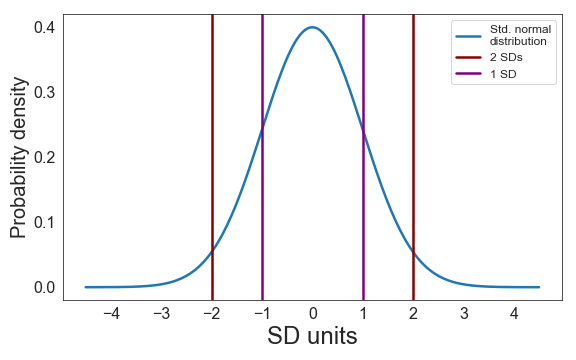
To identify the SD of a standard normal distribution on a graph, find the inflection points (i.e., the points where the slope of the distribution stops increasing or stops decreasing). An intuitive explanation for understanding inflection points is this: Imagine the standard normal distribution shown above is a road on a map (i.e., you’re looking down on it). Now imagine you drive along this road from west to east in a car. To take the first bend you need to turn the steering wheel counter-clockwise. To take the northern bend you clearly have to turn your steering wheel clockwise. Thus, there must be one point between these two bends where you’re going straight ahead (if only for the briefest of moments) - this is the inflection point.
To make it easier to identify these points exactly, one can plot the first derivative of the standard normal distribution (i.e., we plot its slope):
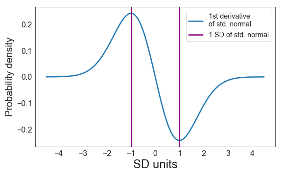
Note that the inflection points of the standard normal distribution correspond to the maximum and minimum values of the derivative, and are located at ± 1 SD of the original distribution.
34.3 The basic logic of null hypothesis significance testing (NHST)
This is the basic logic of NHST:
- You assume there is no effect (i.e., you formulate a null hypothesis)[^You can also hypothesise that there is a certain effect, but this is quite rare.]
- You ask “If I assume there is no effect, what is the probability of finding the effect that I found (or a more extreme one)?”
If this probability (your p-value) is sufficiently small (typically below .05 or 5%), you say that your result is significant. “Significant” means that the observed effect is so unlikely to have arisen by chance that you decide to reject the null hypothesis. If your result is not significant (i.e., the p-value is somewhere between 1 and .05), you say that you have failed to reject the null hypothesis.
How do we know how (im)probable a certain effect is? This depends on only two things:
- The variability in the sample (which is used to estimate the variability in the population, which is usually unknown).
- The sample size.
We can use these two pieces of information to construct a distribution that represents the probability of all possible outcomes under the assumption that the null hypothesis is true38. This distribution is the so-called sampling distribution. Intuitively, if you assume there is no effect, actually finding no or a rather small effect should be quite likely, whereas finding a large effect should be quite unlikely. This intuition is reflected in the shape of the sampling distribution: It’s a normal distribution39.
To construct a normal distribution, one only needs to know two things: Its mean and standard deviation. The mean of the sampling distribution is typically 0 (if the null hypothesis is that there is no difference). The standard deviation of the sampling distribution (often referred to as the standard error, SE) is calculated as follows:
\[SD_{sampling\ distribution} = SE_{mean} = \frac{SD_{sample}}{\sqrt{N}}\]
The basic logic here is the following:
- If there is a lot of variability in your population, there will also be more variability in the sampling distribution → finding a significant p-value will be more difficult
- If you have a small sample, there will also be more variability in the sampling distribution → finding a significant p-value will also be more difficult
Inferential statistics involves converting the empirically observed effect (e.g., a mean interference effect of 10 ms) to a location on the sampling distribution (we basically check how probable our outcome or a more extreme outcome was under the assumption that the null hypothesis is true). This is done by standardising (simply because this makes the calculations easier). As mentioned above, a standard normal distribution has a mean of 0 and a standard deviation of 1. The z-value (or t-value) we compute is the effect we found converted to standard deviation units on the sampling distribution.
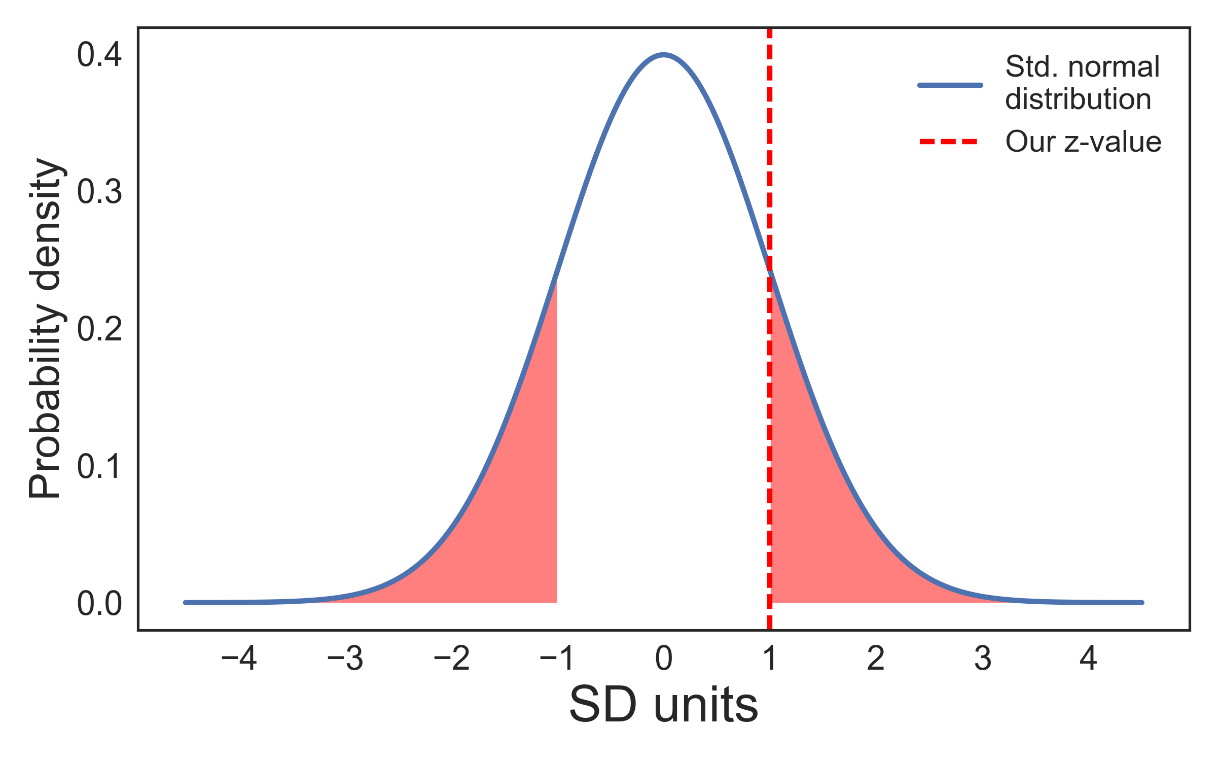
A z-value of 1 would mean that our effect was one standard deviation away from the mean of the sampling distribution. If we were to collect many samples from our population and the null hypothesis were true, we would get a z-value of 1 or higher in 32% of our samples (remember that 68% of the values lie between ±1 SD). That is, this would happen quite frequently. Therefore, we would not consider such a result significant.
The graph shows that 32% of the area of the curve are located outside ±1 SD:
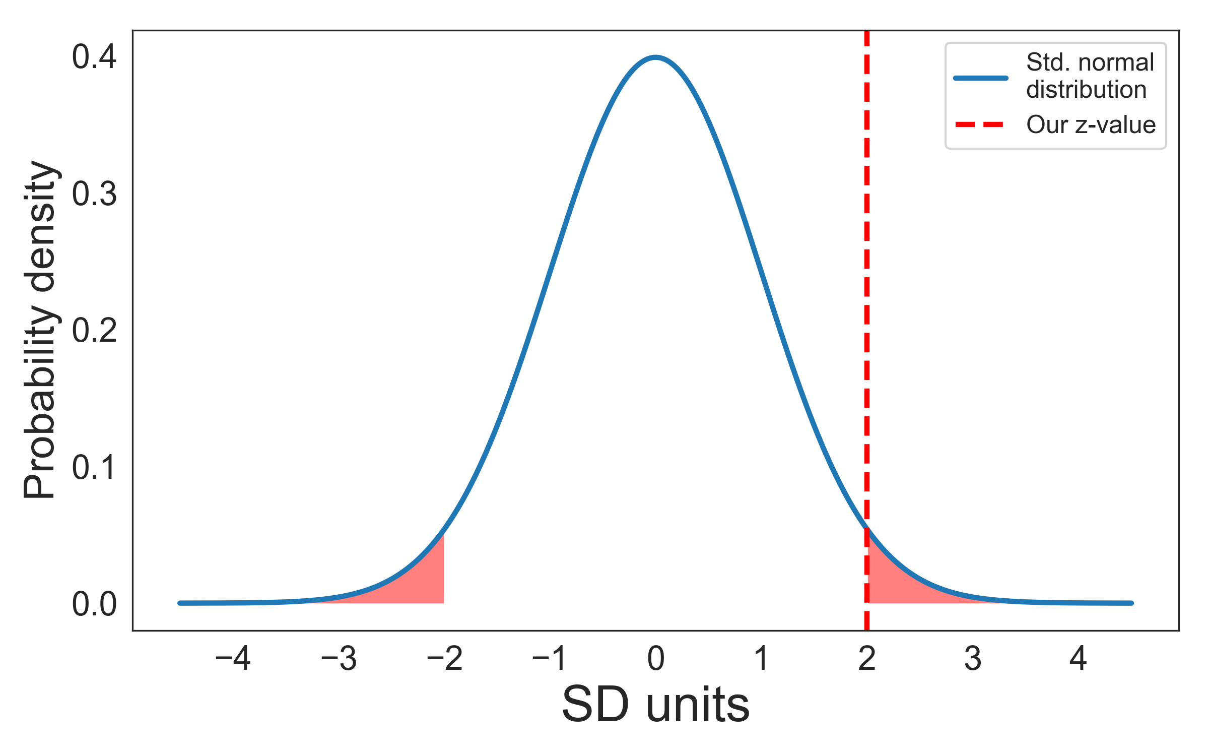
A z-value of 2 would mean that our effect was two standard deviations away from the mean of the sampling distribution. If we were to collect many samples from our population and the null hypothesis were true, we would get a z-value of 2 or higher in 5% of our samples (remember that about 95% of the values lie between ±2 SDs). Remember that 5% is the most frequently used \(\alpha\)-value. Thus, if our z-value were 2 or above, the result would be considered significant (in the sense of unlikely to have occurred by chance under the assumption of the null hypothesis being true).
The graph shows that about 5% of the area of the curve are located outside ±2 SDs:
If your result is not significant, do not say that you accept the null hypothesis (more information here and here) or, Heaven forbid!, that you showed that the null hypothesis is true. Using NHST, you cannot provide evidence for the null hypothesis. This is in fact one of the reasons why Bayesians have been arguing against the use of NHST. You can find out more information about this debate here.
To reiterate, the p-value is the probability of finding an effect at least as extreme as the one you found under the assumption that the null hypothesis is true. The p-value is not the probability that the null hypothesis is actually true, and \((1-p)\) is not the probability that the alternative hypothesis is true. A number of misconceptions concerning p-values, confidence intervals, and power are discussed in this article.
At present, the APA Publication Manual does not actively discourage the use of NHST (although at least one psychology journal has banned it!), but it recommends to complement its use with the reporting of effect sizes and confidence intervals.
34.4 Distributions of participant means vs. sampling distributions
Please note that we now have two types of distributions that are assumed to be normally distributed: The distribution of our participant means and the sampling distribution. Keep in mind the difference between two types of distributions:
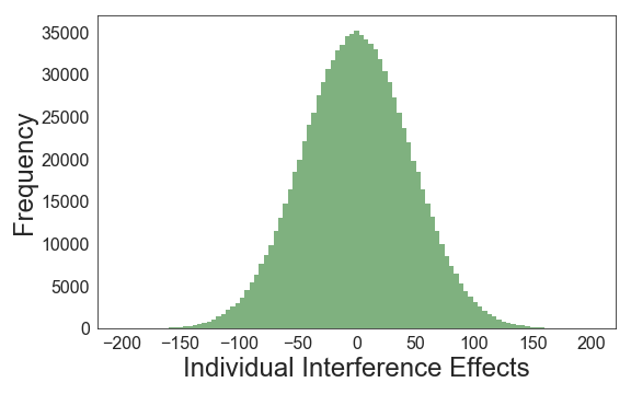
The data points for your distribution of participant means come from individual participants. That is, once you have calculated the means for all your participants (e.g., their mean interference effect), you can plot a histogram showing this distribution. In this distribution, data point 1 will be the size of the interference effect in participant 1 (e.g., 40 ms), data point 2 will be the size of the interference effect in participant 2 (e.g., 15 ms), and so on.
We can simulate such a distribution for 1,000,000 participants. For the simulation, we assume that the null hypothesis is true (i.e., we assume there is no interference effect), and we also assume that the standard deviation of the interference effects is 50 ms. This is the distribution of interference scores we get:
The second type of distribution is the sampling distribution. This distribution no longer has participants as data points, but sample means. The basic idea is that now you’re drawing many, many samples from your population. For each of the samples you’re going to calculate the mean interference effect in the sample. Say, you were to draw samples of 10 participants (note that the participant labels simply refer to the order in which the participants were drawn; P1 in Sample 1 and P1 in Sample 2 are most likely different participants):
| Participants | Sample 1 | Sample 2 | Sample 3 | … |
|---|---|---|---|---|
| P1 | 71 | 62 | -37 | … |
| P2 | -6 | 15 | 49 | … |
| P3 | 50 | 11 | -7 | … |
| P4 | 29 | -1 | -37 | … |
| P5 | -9 | -10 | -8 | … |
| P6 | -44 | -13 | 81 | … |
| P7 | -20 | -32 | -8 | … |
| P8 | -33 | 102 | -34 | … |
| P9 | -57 | -60 | 65 | … |
| P10 | -45 | -15 | 17 | … |
| Mean | -7 | 6 | 8 | … |
The data points for your sampling distribution are the sample means (-7, 6, 8, …). Note that based on our sample, we sometimes underestimate the true interference effect (which we know to be 0 because that is our assumption), and sometimes overestimate the true interference effect. That is, there is some variability to our estimates of the true mean. In fact, we can quite easily calculate the standard deviation we are going to find in our sampling distribution - it is the standard error:
\[{SE_D = \frac{s_D}{\sqrt{N}} = \frac{50}{\sqrt{10}}} = 15.8\]
In words: The standard deviation of the sampling distribution of the mean RT differences is the standard deviation of the difference scores in our sample divided by the square root of \(N\).
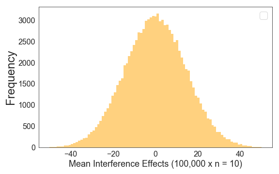
Note the standard deviation in our sampling distribution (15.8) is much smaller than the standard deviation in our original distribution of values (which was 50). If we draw 100,000 samples with a sample size of 10 from our simulated population, this is the distribution of mean differences under the assumption that the null hypothesis is true:
Now, let’s try this with a sample size of 176. If we draw 100,000 samples, we get this distribution (note that the x-axis range is much smaller as compared to an N of 10):
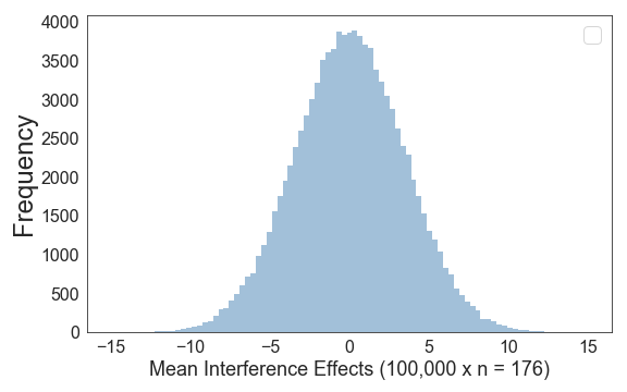
As expected, most frequently our sample mean is pretty close to the population mean of 0, but sometimes our estimate is a bit off.
We can also directly compare the sampling distributions under the null hypothesis for n’s of 10 and 176:
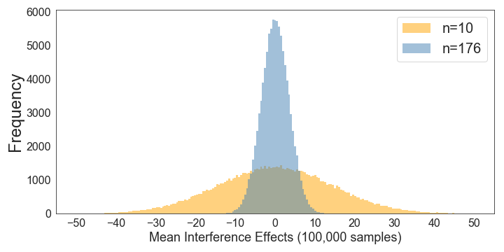
This makes it very clear how a larger sample size reduces the size of the standard deviation of the sampling distribution. Note how this means that increasing the sample size will allow you to find a significant effect more easily, even if there is no change in the size of your experimental effect (i.e., if the interference is constant at 50 ms).
Note that both of these distributions fit a t-distribution40 extremely well:
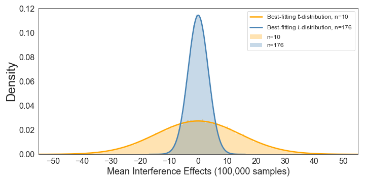
As an aside, please note that this also shows that one cannot evaluate the kurtosis of a distribution without a fitted t-distribution or normal distribution being displayed!
In accordance with the excellent fit, when we standardise both distributions by dividing each value in each distribution by the standard deviation of the respective sampling distribution, we get basically identical distributions:
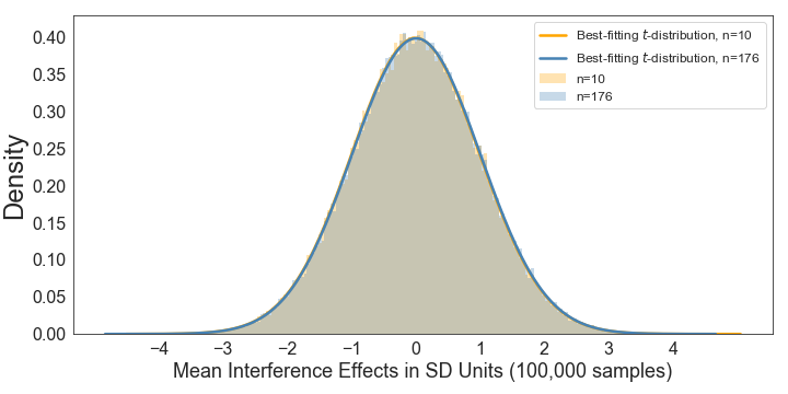
This is what standardisation does for you. As a result, you can now use online tools to calculate the p-value that corresponds to a given t-value, no matter what the standard deviation or the sample size in the respective samples were.
Note that this is an assumption you make. You do not know if the null hypothesis is really true or not.↩︎
For smaller samples, its shape will follow a t-distribution.↩︎
The t-distribution is very similar to a normal distribution. For small n’s, it has slightly heavier tails. This means that more extreme outcomes are slightly more likely. As a result of this, with a small n one would need to find a slightly larger interference effect for it to become significant. For larger n’s (say, 50 or more participants), the t-distribution is practically identical to the normal distribution.↩︎