Chapter 37 The Pearson correlation test
This week, we are going to cover how to run a Pearson correlation test using SPSS. As running the test is again relatively straightforward, we will once more focus on understanding the output and manually doing a correlation test in Excel. We will also show you to how to report the correlation test in a lab report following APA style.
The Pearson correlation test investigates if the association between two variables is significantly different from an association expected under the null hypothesis. Typically, the association expected under the null will be 0. For us, the Pearson correlation test will find out if the interference scores for the flanker task and the Stroop task are significantly correlated.
Please download this SPSS data file and open it.
Please note that we will again be using a relatively small set of data with no outliers as this will make the subsequent step-by-step analyses in Excel easier.
37.1 Running the Pearson correlation test
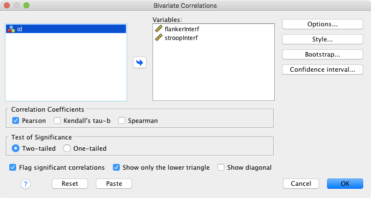
To run the Pearson correlation test in SPSS, go to Analyze → Correlate → Bivariate. Add the variables you would like to correlate to Variables (order is not relevant). We are solely going to focus on the parametric Pearson correlation coefficient, not on the non-parametric correlation coefficients Kendall’s tau-b and Spearman’s \(\rho\). We select the following options:
- Tick “Show only lower triangle”
- Untick “Show diagonal”
This reduces the amount of redundant/uninformative output. Thus, our primary setup for the correlation analysis should look like this:
In addition, we have the following options:
- Options
- Statistics: Typically, we will not need these.
- Missing Values
- This is only relevant if you have more than two variables.
- Exclude cases pairwise (approach might also be referred to as task-wise): A case that has a missing value for one variable (say, variable A) will still be included in correlations not involving this variable (e.g., correlation between variables B and C) → thus, you might have different n’s for your correlations.
- Exclude cases listwise (approach might also be referred to as case-wise): As soon as there is one value missing, the participant will be excluded from all correlations → this ensures that the same participants are included in all correlations.
- Style: Not currently of interest.
- Bootstrap: Not currently of interest.
- Confidence interval
- Select “Estimate confidence interval of bivariate correlation parameter”.
- Leave default for other values (annoyingly the SPSS documentation does not further specify the “bias adjustment”).
If you cannot see the “Confidence interval” option, please make sure to install the latest Fix Pack for your operating system. You can download the Fix Packs here.
37.2 The Pearson correlation test output
This is the output of our analysis:
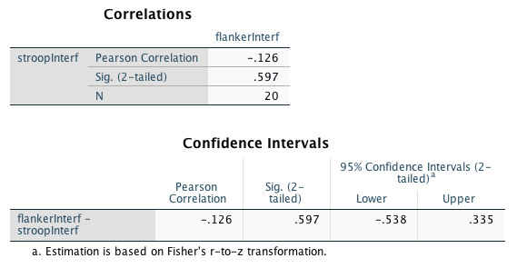
The “Correlations” table has the following information:
- The correlation coefficient r (“Pearson Correlation” in the table).
- The p-value (“Sig. (2-tailed)” in the table).
- And here comes the catch: While SPSS reports the degrees of freedom for the t-test, it does report the sample size N for the correlation analysis. In your lab report, you will need to include the degrees of freedom. These are calculated as \(N-2\).
The “Confidence Intervals” table repeats the r-value and the p-value and, more importantly, reports the lower and upper confidence interval limits.
37.3 What does the output mean?
Pearson’s correlation coefficient can vary between -1 and 1, where -1 is a perfect negative correlation, 1 is a perfect positive correlation, and 0 indicates no correlation between the variables. This is the formula to compute r for two variables \(x\) and \(y\):
\[r_{xy} = \frac{\Sigma_{i=1}^N(x_i-\overline{x})(y_i-\overline{y})}{\sqrt{\Sigma_{i=1}^N(x_i-\overline{x})^2}\sqrt{\Sigma_{i=1}^N(y_i-\overline{y})^2}}\]
In words:
- Numerator
- Subtract the mean of variable \(x\) from each participant’s value for \(x\) → \((x_i-\overline{x})\)
- Subtract the mean of variable \(y\) from each participant’s value for \(y\) → \((y_i-\overline{y})\)
- Multiply the differences for each participant → \((x_i-\overline{x})(y_i-\overline{y})\)
- Sum up the results of the multiplications across participants → \(\Sigma_{i=1}^N\)
- Denominator
- Subtract the mean of variable \(x\) from each participant’s value for \(x\) and square the result → \((x_i-\overline{x})^2\)
- Calculate the sum of squares for \(x\) → \({\Sigma_{i=1}^N(x_i-\overline{x})^2}\)
- Calculate the square root of the sum of squares for \(x\)
- Subtract the mean of variable \(y\) from each participant’s value for \(y\) and square the result → \((y_i-\overline{y})^2\)
- Calculate the sum of squares for \(y\) → \({\Sigma_{i=1}^N(y_i-\overline{y})^2}\)
- Calculate the square root of the sum of squares for \(y\)
- Multiply the two square roots
- Divide the numerator by the denominator
But how do we get the p-value for the Pearson correlation coefficient? The basic idea is the same as for the t-test: If there is no correlation between the variables (i.e., if our null hypothesis were true), what sort of correlations would we expect to get by chance? Then, we again ask: Given this distribution of correlations under the null hypothesis, what was the probability of finding the correlation that we found (or a more extreme one)?
Under the null hypothesis of there being no correlation between variables, the sampling distribution of correlations expected under the null hypothesis is approximately normal. In fact, it closely approximates a t-distribution with \(N-2\) degrees of freedom. The SE for this sampling distribution of r is calculated in the following way:
\[SE_r = \frac{\sqrt{1-r^2}}{\sqrt{N-2}} = \sqrt{\frac{1-r^2}{N-2}}\]
In our example (the sign of the correlation is irrelevant for the following calculations):
\[SE_r = \sqrt{\frac{1 - .126^2}{20-2}} = 0.234\]
We can then calculate the t-value:
\[t = \frac{r}{SE_r} = \frac{.126}{0.234} = 0.538\]
(It is one of the weird coincidences in this magical universe that this value is identical to the absolute value of the lower CI limit. There could be an infinite number of parallel universes where this was not the case.)
Now that we have the t-value, we can finally calculate the p-value. Once again, we can look this up using an online calculator. For our example, we get a p-value of .597. This is clearly above .05, thus our correlation is not significant. (Once again, please note that this matches the result from SPSS.)
Again, the calculation of the confidence intervals is something we will not cover in this lab class. If you are interested in how exactly these are calculated, you can look this up here.
37.4 Lab 14 exercise
In this exercise, you will compute a correlation test step by step. We have provided you with an example using the same data as in the SPSS file. First, make sure you understand the individual steps of the analysis. Then, compute your own correlation test using IDs 24 to 45. Check your result by copying the values into SPSS and running a correlation test on them.
We will go through these steps in the lab class.
Please download this Excel file and open it.
Here is a video of me completing the exercise:
37.5 The effect size for a Pearson correlation test
Conveniently, r is an effect size. A correlation coefficient describes a particular strength of relationship, no matter if it is based on 20 or 200 participants. Therefore, we don’t need to compute a separate effect size measure. Here is a nice correlation coefficient visualisation illustrating this.
37.6 Reporting the results of a Pearson correlation analysis
For lab reports:
«The interference effects in the flanker task and the Stroop task were not significantly correlated, r(18) = -.126, p = .597, 95% CI [-.538, .335].»
This of course assumes that you have already reported the relevant means and SDs at this point.